Complete Solution for SQL Based Real Time Streaming Analytics & Machine Learning

 

This hypothetical and high level architecture diagram will explain how we can use OSS technologies more effectively. We are going to discuss about this whole solution under four main subject areas.

1. Distributed Streaming Message Broker (Data Pipeline)
2. Streaming ETL & Streaming Aggregation
3. Time Series Data Storing & ML Processing
4. Dashboard & Notification 

Distributed Streaming Message Broker

We use Kafka as our data pipeline, you can get more details about Kafka from here [1] .
Kafka is proven technology which perform as distributed streaming log. Using it's partitioning technique we can scale up easily. It's perfectly ideal for event driven architecture because it's streaming nature. Kafka make it much more likely that disk access is often sequential and it utilized OS page cache efficiently [2].

Streaming ETL & Streaming Aggregation

Flink will be the stream processing platform that we use for aggregation, ETL and CEP. Flink by-design support stream processing and it's widely use streaming technology at the moment. Flink is based on the DataFlow model which means, Flink is processing the elements as and when they come rather than processing them in micro-batches (which is done by Spark streaming).

Uber AthenaX is a SQL based streaming analytics framework [3]. It's combination of YARN , Calcite & Flink. AthenaX give APIs to monitor, access & administrate life cyclone of Flink Jobs. Also because of Calcite we can write SQL based stream processing applications and run them inside AthenaX easily.

Time Series Data Storing & ML Processing

We use Cassandra as time series data storage. Cassandra architecture is ideal for this purpose because of sequential writing to disk, which will help for fast reading large set of data.

So the time series prepared data we got from streaming analytics platform, will be stored in Cassandra for machine learning.

We will train several ML models using prepared data, then trained models/knowledge base will be stored (as binary) in Cassandra.This way we can dynamically select trained models when we analyze real time data.

Spark slave/worker and Cassandra will reside in same host, and both will be connected by Spark-Cassandra-Connector. For high availability there will be active and stand by Spark master while Zookeeper keep the state of each master.

The main advantage of this approach is  guarantee of data locality between Cassandra node and Spark slave, which will cause for high performance data fetching.

Dashboard & Notification

Finally you need to store analyzed data for later use (Dashboard & trend analysis). Say for example, If we use this solution for predictive analysis, you can save predicted data in ElasticSearch. By using ELK stack, people can create Dashboards easily using analysis data with Kibana.

Also there are lot of other features in ElasticSearch & Kibana such as ES alerts, Trend analysis, Searching and etc...


References:

[1] https://kafka.apache.org/
[2] https://stackoverflow.com/questions/45751641/how-does-kafka-guarantee-sequential-disk-access
[3] https://eng.uber.com/tag/athenax/
[4] https://www.infoq.com/presentations/uber-ml-architecture-models?utm_source=infoqemail&utm_medium=ai-ml-data-eng&utm_campaign=newsletter&utm_content=05152018

Spark Cassandra Integration with spark-cassandra-connector

In here, I am going to show how to integrate local single node Cassandra db with standalone spark using spark-cassandra-connector.

Setup Cassandra, Spark, Scala & ScalaBuildTool

1. Download Cassandra & Spark. I am using Cassandra version 3.11.2  and Spark version 2.2.1 .

http://cassandra.apache.org/download/
https://spark.apache.org/releases/spark-release-2-2-1.html
https://www.scala-lang.org/download/2.11.8.html
https://www.scala-sbt.org/download.html

2. Environment setup in .profile

#cassandra setup
export CASSANDRA_HOME=/home/dhanuka/software/apache-cassandra-3.11.2

#spark, sbt and scala setup
export SPARK_HOME=/home/dhanuka/software/spark/spark-2.2.1-bin-hadoop2.7
export SBT_HOME=/home/dhanuka/software/spark/sbt-launcher-packaging-0.13.13
export SCALA_HOME=/home/dhanuka/software/scala-2.11.8

PATH=$PATH:$JAVA_HOME/bin:$MAVEN_HOME/bin:SPARK_HOME/bin:$SBT_HOME/bin:$SCALA_HOME/bin:CASSANDRA_HOME/bin

3. $ source ~/.profile 

Create Cassandra Keyspace and Table

 1. Start cassandra with following command

$ cassandra -f

2. Start CQL shell

$ cqlsh

3. Create keyspace and a table

cqlsh> CREATE KEYSPACE people WITH replication = {'class': 'SimpleStrategy', 'replication_factor':1};

cqlsh> use people;

cqlsh:people> CREATE TABLE users(
          ... id varchar ,
          ... first_name varchar,
          ... last_name varchar,
          ... city varchar,
          ... emails varchar,
          ... PRIMARY KEY (id));
 
cqlsh:people>  Insert into users (id,first_name,last_name,city,emails) values('1','dhanuka','ranasinghe','colombo','dhanuka.priyanath@gmail.com');

 cqlsh:people> select * from users;

 id      | city    | emails                      | first_name | last_name
---------+---------+-----------------------------+------------+------------
 1 | colombo | dhanuka.priyanath@gmail.com |    dhanuka | ranasinghe




Build spark-cassandra-connector.

1. clone from git hub repository.

$  git clone https://github.com/datastax/spark-cassandra-connector.git 

$  cd spark-cassandra-connector

2. Build the project with scala 2.11 and cassandra 3.11.2

$  spark-cassandra-connector$ sbt -Dscala-2.11=true -Dtest.cassandra.version=3.11.2 assembly

You can find the jar location below.

$  spark-cassandra-connector/spark-cassandra-connector/target/full/scala-2.11/spark-cassandra-connector-assembly-2.0.7-82-g0369a7b.jar

$  mv  spark-cassandra-connector-assembly-2.0.7-82-g0369a7b.jar   spark-cassandra-connector-assembly-2.0.7.jar


 Connect Spark with Cassandra through Spark-Shell

1. Copy cassandra-connector-assembly-2.0.7.jar to spark jars location. Copy to below location

$  cp cassandra-connector-assembly-2.0.7.jar  $SPARK_HOME/jars

2.  Start spark-shell

$ spark-shell --jars $SPARK_HOME/jars/spark-cassandra-connector-assembly-2.0.7.jar

3. Stop current spark context

scala> sc.stop

4. Program to read Cassandra from spark

scala> import com.datastax.spark.connector._, org.apache.spark.SparkContext, org.apache.spark.SparkContext._, org.apache.spark.SparkConf
import com.datastax.spark.connector._
import org.apache.spark.SparkContext
import org.apache.spark.SparkContext._
import org.apache.spark.SparkConf


scala> val conf = new SparkConf(true).set("spark.cassandra.connection.host", "localhost")
conf: org.apache.spark.SparkConf = org.apache.spark.SparkConf@2c2a7d53

scala> val sc = new SparkContext(conf)
sc: org.apache.spark.SparkContext = org.apache.spark.SparkContext@15914bb5

scala> val test_spark_rdd = sc.cassandraTable("people", "users")
test_spark_rdd: com.datastax.spark.connector.rdd.CassandraTableScanRDD[com.datastax.spark.connector.CassandraRow] = CassandraTableScanRDD[0] at RDD at CassandraRDD.scala:19

scala> test_spark_rdd.first
res1: com.datastax.spark.connector.CassandraRow = CassandraRow{id: 1, city: colombo, emails: dhanuka.priyanath@gmail.com, first_name: dhanuka, last_name: ranasinghe}

References:

[1] https://www.datastax.com/dev/blog/kindling-an-introduction-to-spark-with-cassandra-part-1

[2] https://www.youtube.com/watch?v=jpEABn80OCU

Simple explanation about basic machine learning algorythms with R

Supervised   

Supervised learning is where you have input variables (x) and an output variable (Y) and you use an algorithm to learn the mapping function from the input to the output.

Y = f(X)

The goal is to approximate the mapping function so well that when you have new input data (x) that you can predict the output variables (Y) for that data.

Regression vs Classification   

Regression is used to predict continuous values. Classification is used to predict which class a data point is part of (discrete value).

                           

Regression

In the case of regression, the target variable is continuous — meaning that it can take any value within a specified range. Input variables, on the other hand, can be either discrete or continuous.

Linear Regression

Math:

SepalLength = a * PetalWidth + b* PetalLength +c

Code:

# Load required packages

library(ggplot2)

# Load iris dataset

data(iris)

# Have a look at the first 10 observations of the dataset

head(iris)

# Fit the regression line

fitted_model <- lm(Sepal.Length ~ Petal.Width + Petal.Length, data = iris)

# Get details about the parameters of the selected model

summary(fitted_model)

# Plot the data points along with the regression line

ggplot(iris, aes(x = Petal.Width, y = Petal.Length, color = Species)) +

 geom_point(alpha = 6/10)  +

 stat_smooth(method = "lm", fill="blue", colour="grey50", size=0.5, alpha = 0.1)

Logistic Regression

The difference is that the regression line is not straight anymore.

Math:

Y=g(a*X1+b*X2)

...where g() is the logistic function.

Code:

# Load required packages

library(ggplot2)

# Load data

data(mtcars)

# Keep a subset of the data features that includes on the measurement we are interested in

cars <- subset(mtcars, select=c(mpg, am, vs))

# Fit the logistic regression line

fitted_model <- glm(am ~ mpg+vs, data=cars, family=binomial(link="logit"))

# Plot the results

ggplot(cars, aes(x=mpg, y=vs, colour = am)) + geom_point(alpha = 6/10) +

 stat_smooth(method="glm",fill="blue", colour="grey50", size=0.5, alpha = 0.1, method.args=list(family="binomial"))

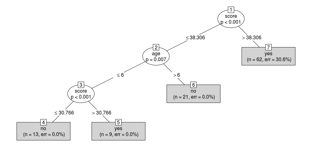
Decision Trees (Classification or Regression)

What they basically do is draw a “map” of all possible paths along with the corresponding result in each case.

Based on a tree like this, the algorithm can decide which path to follow at each step depending on the value of the corresponding criterion.

Code:

# Include required packages

#install.packages("party")

#install.packages("partykit")

library(party)

library(partykit)

# Have a look at the first ten observations of the dataset

print(head(readingSkills))

input.dat <- readingSkills[c(1:105),]

# Grow the decision tree

output.tree <- ctree(

 nativeSpeaker ~ age + shoeSize + score,

 data = input.dat)

# Plot the results

plot(as.simpleparty(output.tree))

Unsupervised

Unsupervised learning is where you only have input data (X) and no corresponding output variables.

The goal for unsupervised learning is to model the underlying structure or distribution in the data in order to learn more about the data.

These are called unsupervised learning because unlike supervised learning above there is no correct answers and there is no teacher. Algorithms are left to their own devises to discover and present the interesting structure in the data.

   

Clustering

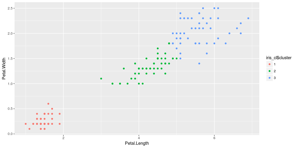
With clustering, if we have some initial data at our disposal, we want to form groups so that the data points belonging to some group are similar and are different from data points of the other groups , such as grouping customers by purchasing behavior..

Algorythm :

1. Initialization step: For k=3 clusters, the algorithm randomly selects three points as centroids for each cluster.
2. Cluster assignment step: The algorithm goes through the rest of the data points and assigns each one of them to the closest cluster.
3. Centroid move step: After cluster assignment, the centroid of each cluster is moved to the average of all points belonging to the cluster.

Steps 2 and 3 are repeated multiple times until there is no change to be made regarding cluster assignments.

Code:

# Load required packages

library(ggplot2)

library(datasets)

# Load data

data(iris)

# Set seed to make results reproducible

set.seed(20)

# Implement k-means with 3 clusters

iris_cl <- kmeans(iris[, 3:4], 3, nstart = 20)

iris_cl$cluster <- as.factor(iris_cl$cluster)

# Plot points colored by predicted cluster

ggplot(iris, aes(Petal.Length, Petal.Width, color = iris_cl$cluster)) + geom_point()

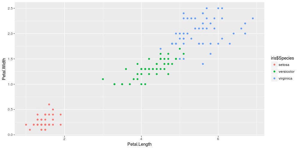
Colored by Species

Code:

# Load required packages

library(ggplot2)

library(datasets)

# Load data

data(iris)

# Set seed to make results reproducible

set.seed(20)

# Implement k-means with 3 clusters

iris_cl <- kmeans(iris[, 3:4], 3, nstart = 20)

iris_cl$cluster <- as.factor(iris_cl$cluster)

# Plot points colored by predicted cluster

ggplot(iris, aes(Petal.Length, Petal.Width, color = iris$Species)) + geom_point()

Association

An association rule learning problem is where you want to discover rules that describe large portions of your data, such as people that buy X also tend to buy Y.

References:

https://dzone.com/articles/3-machine-learning-algorithms-you-need-to-know?edition=329502&utm_source=Weekly%20Digest&utm_medium=email&utm_campaign=Weekly%20Digest%202017-10-04

https://machinelearningmastery.com/supervised-and-unsupervised-machine-learning-algorithms/